DATE: 2026-05-24

Subject: Theoretical Application of a Combined Graph Convolutional Network (GCN) and Long Short-Term Memory (LSTM) Framework to Enhance Network Observability

Executive Summary

Modern network architectures, from public cloud environments to industrial sensor networks, have grown into complex, dynamic, and distributed systems. This complexity challenges traditional monitoring approaches, which often focus on individual component metrics and fail to capture the emergent behaviors and subtle performance degradations that define contemporary operational issues. To address this, the paradigm of network observability has emerged, shifting the focus from simple data collection to deep, inferential understanding of a system’s internal state through the analysis of its external outputs.

This report presents a theoretical and architectural framework for enhancing network observability by applying a hybrid deep learning model that combines Graph Convolutional Networks (GCNs) and Long Short-Term Memory (LSTM) networks. The GCN+LSTM model is uniquely suited to the challenges of modern networks by its inherent ability to process data that is both structurally and temporally complex.

The core of this approach lies in modeling the network and its telemetry data as a dynamic graph, where network entities (e.g., services, hosts, sensors) are nodes and their interactions are edges. GCNs analyze the spatial dimension of this data, capturing the intricate dependencies and relational patterns across the network topology at a given moment. LSTMs analyze the temporal dimension, modeling how these patterns evolve over time.

This report details the application of this framework to two primary, high-impact use cases:

1. Anomaly Detection: Moving beyond single-metric thresholding to identify complex, system-wide anomalies that manifest as deviations from learned normal spatiotemporal patterns. Research demonstrates this approach can achieve precision and recall rates approaching 0.90 for detecting subtle, chronic failures in complex cloud systems.

2. Network Performance Prediction: Proactively forecasting key performance indicators (KPIs) and path performance metrics (PPMs) such as latency, congestion, and packet delivery ratio. This enables intelligent routing, proactive resource scaling, and congestion control, with studies showing significant improvements in prediction accuracy over state-of-the-art methods.

By synthesizing spatial and temporal dynamics, the GCN+LSTM framework provides a powerful tool for operational inference. It transforms raw telemetry streams into actionable insights, enabling engineering teams to move from a reactive to a proactive operational posture. This document provides the foundational knowledge, architectural design, and evidence-based justification for considering the GCN+LSTM model as a cornerstone of a next-generation network observability strategy.

1. Formalizing Network Observability in the Modern Era

The term “network observability” represents a critical evolution from traditional network monitoring. While monitoring is concerned with collecting and displaying metrics (what is happening), observability is concerned with inferential analysis to understand why it is happening. It is the practice of inferring the internal state, health, and performance of a complex system by analyzing the telemetry data it generates.

Synthesizing from contemporary research, network observability in the context of large-scale distributed systems can be formally defined as:

A system property and a technical practice wherein the internal operational state of a network is inferred through the comprehensive analysis of external telemetry data (e.g., metrics, logs, traces). It goes beyond tracking individual Key Performance Indicators (KPIs) to enable joint judgments based on the synergistic, spatiotemporal relationships among distributed components, thereby facilitating the discovery of hidden systemic states and the prediction of future behavior.

This definition is predicated on several core principles derived from the challenges of modern network environments:

• Rejection of Siloed Analysis: In architectures such as microservices, industrial IoT (IIoT), or Vehicular Ad Hoc Networks (VANETs), the status of the system cannot be determined by examining individual components in isolation. An issue in one service may only become apparent through its subtle, cascading effects on downstream services. Observability requires modeling the entire system and its interconnections (Yu et al., 2023).
• Embrace of Dynamic Topology: Unlike static, monolithic systems, modern networks exhibit dynamic topologies where connections and even components themselves are ephemeral. Observability must account for these structural changes over time, capturing not just how node properties change but how their relationships evolve (Yu et al., 2023).
• Focus on Operational Inference: The ultimate goal of observability is not data collection but actionable inference. This includes core tasks like network tomography—the inference of unobserved network characteristics from observed measurements—as well as fault diagnosis, performance prediction, and automated traffic control (Hu et al., 2025). For example, by measuring end-to-end path performance metrics (PPMs) like latency for a subset of paths, a robust observability model can infer the latency for all other paths in the network.
• Detection of “Chronic” Failures: Modern, resilient systems often do not fail catastrophically. Instead, they suffer from “gradual, chronic, localized failures or quality degradations” (Yu et al., 2023). These subtle issues, such as a slight increase in packet loss or a minor rise in service latency under specific load conditions, are often invisible to traditional monitoring but are prime targets for an observability framework capable of detecting faint deviations from complex, normal behaviors.

In essence, network observability demands a transition from collecting data points to understanding data patterns within a holistic, dynamic context.

2. Modeling Network Telemetry as Graph-Structured Temporal Data

The power of the GCN+LSTM framework stems from its natural alignment with the structure of network telemetry data. A modern network is fundamentally a graph, and its behavior is a time series. By formally mapping observability data into this structure, we unlock the ability to apply advanced spatiotemporal modeling.

2.1 The Graph Data Model

At any given time step t, the state of a network can be represented as a property graph, G_t, consisting of nodes, edges, and their associated features.

• Nodes (Vertices): Nodes represent the core entities of the network. Their definition is use-case dependent:
  • In a cloud infrastructure, nodes can be microservices, containers, pods, virtual machines, or physical hosts (Yu et al., 2023).
  • In an Industrial IoT (IIoT) context, nodes are sensors, actuators, controllers, or gateways (Yang et al., 2025).
  • In a communication network, nodes represent routers, switches, or other network hardware.
• Node Features: Each node possesses a set of attributes, represented as a feature vector. These are typically the KPIs collected from the entity. Examples include:
  • CPU and memory utilization
  • Disk I/O rates
  • Sensor readings (e.g., temperature, pressure)
  • Queue depth or buffer utilization
• Edges (Connections): Edges represent the interactions, communication pathways, or logical relationships between nodes. The existence of an edge signifies a dependency.
  • In a microservices application, an edge could represent an API call from one service to another.
  • In an IIoT network, an edge could be derived from a Spearman correlation matrix, indicating a strong statistical relationship between the readings of two different sensors (Yang et al., 2025).
  • In a computer network, an edge represents a physical or logical link.
• Edge Features: Like nodes, edges can have their own feature vectors describing the nature of the interaction.
  • Communication volume (e.g., requests per second, data transferred)
  • Communication latency or response time
  • Packet loss rate
  • Protocol type

This data can be structured into matrices suitable for machine learning: a Node Feature Matrix (X), where each row corresponds to a node’s features, and an Adjacency Matrix (A), which defines the connectivity between nodes.

2.2 The Temporal Dimension

A single graph snapshot provides a spatial view of the network at one instant. However, the most critical insights come from observing how this graph evolves. The state of the network at time t is deeply dependent on its state at t-1, t-2, and so on.

By collecting these graph snapshots at regular intervals, we create a sequence of graphs: [G_{t-k}, ..., G_{t-1}, G_t]. This sequence represents the dynamic, spatiotemporal behavior of the network, capturing both the changing properties of nodes/edges and the potential for the graph’s topology itself to change.

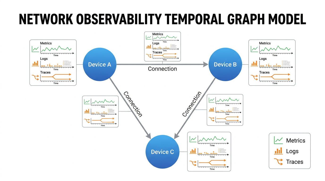Figure 1: Conceptual mapping of network state over time to a sequence of graph snapshots, forming the basis for spatiotemporal analysis.

2.3 Mapping to the GCN+LSTM Framework

This graph-structured temporal data model is precisely what the GCN+LSTM architecture is designed to process. The two components work in concert:

1. GCN for Spatial Feature Extraction: For each graph snapshot G_t in the sequence, a GCN is used to process the graph structure. The GCN generates an embedding (a dense vector representation) for each node by aggregating feature information from its local neighborhood. This process effectively encodes the spatial context of each node—its state relative to the nodes it is connected to. The output of this stage is a sequence of spatially-aware graph embeddings.

2. LSTM for Temporal Feature Extraction: The sequence of graph embeddings produced by the GCN is then fed into an LSTM. The LSTM is renowned for its ability to model long-range dependencies in sequential data. It processes the sequence of graph states, learning the temporal patterns of how the network evolves from one state to the next.

This dual approach allows the model to learn complex, high-level spatiotemporal features that are impossible to capture with methods that treat metrics as independent time series or analyze a network graph statically. It directly models the core principle of observability: that system behavior is an emergent property of interconnected components evolving through time.

3. Primary Observability Use Cases

The GCN+LSTM framework supports a range of operational inference tasks. This report focuses on two primary use cases—anomaly detection and performance prediction—that offer significant value to network engineering and architecture teams.

3.1 Use Case 1: Advanced Anomaly Detection

Traditional anomaly detection, often relying on statistical methods like PCA or single-variate time-series models, is ill-equipped for the complexity of modern systems. It struggles to distinguish between benign fluctuations and genuine, subtle incidents that arise from multi-component interactions.

3.1.1 Problem Scope

Anomalies in distributed systems are rarely simple crashes. More common and insidious are issues like:

• A “gray failure” where a service is running but operating at a degraded performance level.
• A cascading slowdown initiated by a resource bottleneck in one component that propagates through a chain of service calls.
• Anomalous behavior that only occurs when specific conditions across multiple, disparate components align.

An example from an Elasticsearch cluster illustrates this: slight increases in client-side latency, when correlated with overlapping resource usage patterns on specific server nodes, can indicate an underlying performance anomaly that is invisible when looking at server KPIs alone (Yu et al., 2023). These are precisely the types of events a spatiotemporal model is designed to find.

3.1.2 The GCN+LSTM Approach

The anomaly detection task is framed as a forecasting problem. The GCN+LSTM model is trained exclusively on historical telemetry data from periods of normal network operation. Its objective is to learn the intricate patterns of “normalcy” and accurately predict the network’s state at the next time step (t+1) based on a sequence of past states (t-k, ..., t).

The detection mechanism is as follows:

1. Training: The model learns a function F that maps a sequence of past graph snapshots to a predicted future snapshot: Ĝ_{t+1} = F(G_{t-k}, ..., G_t).
2. Inference: During live operation, the model continuously makes predictions.
3. Anomaly Scoring: The predicted graph snapshot Ĝ_{t+1} (containing predicted node/edge features) is compared to the actual, measured graph snapshot G_{t+1}. A reconstruction error or prediction error is calculated.
4. Thresholding: If this error exceeds a predefined, statistically derived threshold, it signifies that the network is behaving in a way that deviates from its learned normal patterns. An alert is triggered.

The GCN captures anomalous spatial patterns (e.g., a node’s CPU is high while a neighbor’s throughput is unexpectedly low), and the LSTM detects anomalous temporal sequences (e.g., this spatial pattern has never occurred following a period of low network-wide latency).

3.1.3 Supporting Evidence

Research provides strong validation for this approach. The AD-DSTL method, which employs a GCN-LSTM architecture for cloud system anomaly detection, was evaluated on four distinct datasets, including a production microservices system with 92 nodes. The model demonstrated superior robustness and a significantly higher F1-score compared to baseline models like standalone GCN, LSTM, and SVM. At higher anomaly levels, both precision and recall reached approximately 0.9, indicating high accuracy and a low false-positive rate (Yu et al., 2023). Similarly, the GCRL model applied to industrial sensor networks improved the F1-score by 4.35% over other state-of-the-art methods, effectively detecting anomalies in water distribution and hydraulic systems (Yang et al., 2025).

3.2 Use Case 2: Network Performance Prediction

Proactive network management depends on the ability to foresee future conditions. Network performance prediction aims to forecast metrics like latency, throughput, and congestion, enabling systems to adapt before performance is impacted. This is a core tenet of network tomography: inferring unobserved or future performance from existing measurements.

3.2.1 Problem Scope

Key challenges in performance prediction include:

• Path-Level Prediction: Predicting the end-to-end performance of a path (e.g., between two services or across a WAN) is more complex than predicting a single node’s state, as it depends on the aggregated performance of all links and nodes along that path.
• Congestion Forecasting: Predicting when and where network congestion will occur is vital for traffic engineering and dynamic routing, especially in highly mobile environments like VANETs where traffic patterns change rapidly.
• Incomplete Knowledge: In many real-world scenarios, the complete network topology or the exact routing paths are unknown or hidden for security reasons. A predictive model should ideally not depend on having complete prior knowledge (Hu et al., 2025).

3.2.2 The GCN+LSTM Approach

For performance prediction, the GCN+LSTM model is trained as a supervised regression model. The objective is to predict a specific target value (or set of values) for a future time step.

The process is as follows:

1. Training: The model is given sequences of past graph snapshots as input and corresponding future performance metrics as labels. For example, the input could be network telemetry from t-k to t, and the label could be the average latency of a specific path at time t+1.
2. Learning:
   • The GCN component learns to create powerful node and path embeddings that implicitly capture topological information and spatial dependencies relevant to performance.
   • The LSTM component learns the temporal dynamics of how traffic patterns and node states evolve to influence future performance.
3. Prediction: Once trained, the model can take a current sequence of telemetry data and output a direct prediction for a future metric (e.g., “congestion level on node X will be 85% in 5 minutes” or “latency on path Y will be 120ms”).

This approach allows for a range of predictive tasks, from node-level KPI prediction to complex, end-to-end path performance metric (PPM) prediction.

3.2.3 Supporting Evidence

A GCN-LSTM model applied to urban VANETs demonstrated its effectiveness in predicting traffic dynamics to enable adaptive routing and congestion control. The hybrid model significantly outperformed benchmarks, achieving a Packet Delivery Ratio (PDR) of 95.0% and reducing prediction errors (Mean Absolute Error of 0.02) far below other methods. This high predictive accuracy translated directly into improved network performance (Maray, 2026). Further, research in network tomography with path-centric graph neural networks (a conceptually similar approach) shows that such models can predict additive metrics like latency with significantly lower error (e.g., a MAPE of 0.6907 on an Internet dataset vs. >0.81 for other methods) without requiring full knowledge of the network topology (Hu et al., 2025).

3.3 Other Potential Use Cases

Beyond these two primary applications, the spatiotemporal features learned by a GCN+LSTM model can be leveraged for other critical observability tasks:

• Automated Root Cause Analysis: By analyzing the attention weights or feature importance within the model following an anomaly detection, it may be possible to automatically identify the nodes, edges, and time points that contributed most significantly to the anomalous prediction, thereby pinpointing the likely root cause.
• Proactive Resource Management: Predictions of future workload or performance degradation can be used to trigger automated remediation actions, such as scaling up cloud resources, diverting traffic, or scheduling preventative maintenance before users are impacted.
• Security Threat Detection: Spatiotemporal anomaly detection can be applied to security-relevant data. An unusual pattern of communication (e.g., a host suddenly communicating with many new internal endpoints) could be flagged as a potential lateral movement attack, even if the individual connections are low-volume.

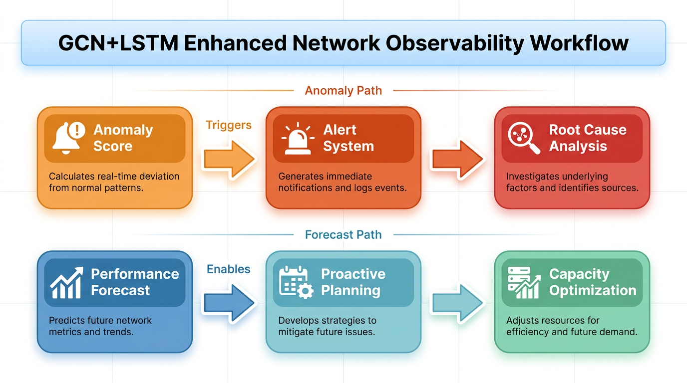Figure 2: The role of GCN+LSTM model outputs in an integrated observability workflow, enabling proactive and automated operational responses.

4. Model Architecture and Foundations

This section details the architectural components, mathematical underpinnings, and evaluation metrics for a GCN+LSTM framework.

4.1 Model Architecture

The GCN+LSTM model is an end-to-end deep learning architecture that processes a sequence of graph snapshots to produce a prediction.

Input: A sequence of k+1 graph snapshots from time t-k to t. Each snapshot consists of a node feature matrix X_i and an adjacency matrix A_i.

Processing Pipeline:

1. Spatial Encoding (GCN): For each time step i in the input sequence, the graph (X_i, A_i) is passed through one or more GCN layers.
   • The GCN aggregates information from neighboring nodes, updating each node’s feature vector to create a spatially aware embedding Z_i. This step is performed for every snapshot in the sequence, producing a sequence of embeddings [Z_{t-k}, ..., Z_t].
2. Temporal Encoding (LSTM): The sequence of node embeddings [Z_{t-k}, ..., Z_t] is fed into an LSTM network.
   • The LSTM processes the sequence step-by-step, maintaining an internal hidden state that captures the temporal dynamics of how the graph evolves. The final hidden state of the LSTM, h_t, represents a compressed spatiotemporal summary of the entire input sequence.
3. Prediction Head (Fully Connected Layer): The final LSTM hidden state h_t is passed to a final feed-forward neural network (the “head”).
   • The structure of this head depends on the task. For anomaly detection, it might aim to reconstruct the input or predict the next graph state. For performance prediction, it will output a regression value. An activation function like Softmax (for classification) or a linear activation (for regression) is used to produce the final output.

Some architectures may employ a dual-LSTM structure, processing node and edge features in separate parallel streams before fusion, to more explicitly model both entity and interaction dynamics (Yu et al., 2023).

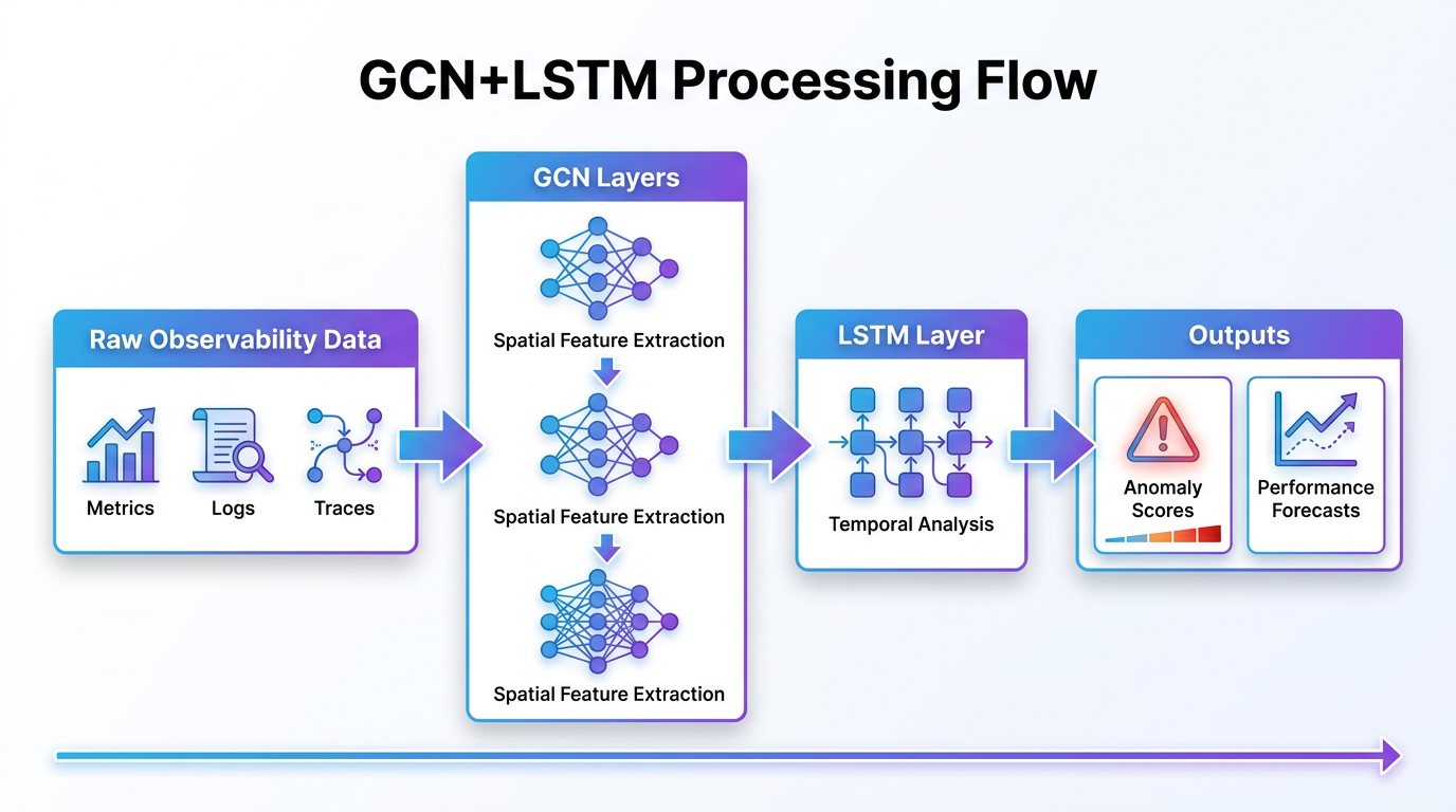Figure 3: Architectural overview of the GCN+LSTM processing pipeline, showing the flow from graph sequences to spatiotemporal encoding and final prediction.

4.2 Mathematical Foundations

Graph Representation

• Adjacency Matrix A: A square matrix of size N x N (where N is the number of nodes) where A_ij = 1 if an edge exists between node i and node j, and 0 otherwise.
• Node Feature Matrix X: A matrix of size N x F (where F is the number of features per node) where row i contains the feature vector for node i.

Graph Convolutional Network (GCN) Layer

The core of the GCN is its propagation rule, which defines how node representations are updated at each layer l. The simplified formula for a GCN layer is:

H⁽ˡ⁺¹⁾ = σ(D̃⁻¹/² Ã D̃⁻¹/² H⁽ˡ⁾ W⁽ˡ⁾)

Where:

• H⁽ˡ⁾ is the matrix of node activations at layer l (H⁽⁰⁾ = X).
• à = A + I is the adjacency matrix A with self-loops added (so a node includes its own features in the aggregation).
• D̃ is the diagonal degree matrix of Ã. The term D̃⁻¹/² Ã D̃⁻¹/² is a symmetric normalization of the adjacency matrix that prevents the scale of feature vectors from exploding and stabilizes the learning process.
• W⁽ˡ⁾ is a trainable weight matrix for layer l.
• σ is a non-linear activation function, such as ReLU (max(0, x)).

In essence, this operation computes a weighted average of the feature vectors of a node and its immediate neighbors. Stacking these layers allows the model to learn representations based on larger neighborhoods.

Long Short-Term Memory (LSTM) Layer

An LSTM is a type of Recurrent Neural Network (RNN) designed to overcome the vanishing gradient problem and learn long-term dependencies. It achieves this through a series of “gates” that control the flow of information. At each time step t, an LSTM cell takes the current input x_t and the previous hidden state h_{t-1} to compute the new hidden state h_t.

This is governed by three gates:

• Forget Gate (f_t): Decides what information to discard from the cell state.
• Input Gate (i_t): Decides which new information to store in the cell state.
• Output Gate (o_t): Decides what part of the cell state to use for the output hidden state.

These gates allow the LSTM to selectively remember relevant information from many time steps in the past while discarding irrelevant information, making it ideal for modeling the temporal evolution of network states.

4.3 Evaluation Metrics

The performance of the GCN+LSTM framework can be assessed using standard machine learning metrics tailored to the specific use case.

For Anomaly Detection (Classification Task):

• Precision: TP / (TP + FP) – Of all the alerts generated, what fraction were actual anomalies? High precision is crucial for building operator trust and avoiding alert fatigue.
• Recall: TP / (TP + FN) – Of all the actual anomalies that occurred, what fraction did the system detect? High recall is critical for ensuring that important events are not missed.
• F1-Score: 2 * (Precision * Recall) / (Precision + Recall) – The harmonic mean of precision and recall, providing a single score that balances the two. It is often the primary metric for evaluating anomaly detectors on imbalanced datasets.

Studies show GCN+LSTM models achieving F1-scores of 95.96% on the WADI industrial control dataset (Yang et al., 2025) and precision/recall around 0.85-0.90 on cloud system datasets (Yu et al., 2023).

For Performance Prediction (Regression Task):

• Mean Absolute Error (MAE): (1/n) * Σ|y_i - ŷ_i| – The average absolute difference between the predicted values (ŷ_i) and the actual values (y_i). It is easily interpretable as it is in the same units as the target variable.
• Root Mean Squared Error (RMSE): sqrt((1/n) * Σ(y_i - ŷ_i)²) – Similar to MAE, but penalizes larger errors more heavily.
• Mean Absolute Percentage Error (MAPE): (100/n) * Σ|(y_i - ŷ_i) / y_i| – Expresses the error as a percentage of the actual value, useful for understanding the relative error.

In VANET performance prediction, a GCN+LSTM model achieved an MAE of 0.02 and an RMSE of 0.07, demonstrating very high predictive accuracy (Maray, 2026). In network tomography tasks, GNN-based approaches reduced MAPE on latency prediction to 0.6907, outperforming baselines that scored over 0.81 (Hu et al., 2025).

5. Conclusion

The GCN+LSTM framework represents a significant theoretical and practical advancement for the field of network observability. By treating network telemetry as dynamic, structured graph data, this approach moves beyond the limitations of traditional monitoring and provides a powerful engine for operational inference. Its proven ability to model the complex, interdependent, and time-varying nature of modern distributed systems makes it exceptionally well-suited for high-value use cases like sophisticated anomaly detection and proactive performance prediction.

While the implementation of such a system requires careful data engineering and model training, the evidence from recent research is compelling. Multiple studies across different domains—cloud computing, industrial control systems, and vehicular networks—have independently reached the same conclusion: the combination of GCN for spatial analysis and LSTM for temporal analysis yields state-of-the-art results.

For technical engineering groups and network architects, this framework offers a clear path toward a more intelligent, automated, and proactive operational model. By adopting a GCN+LSTM approach, organizations can enhance their ability to understand and control their increasingly complex network environments, improve system reliability, and optimize performance in ways that are unattainable with conventional methods. This report provides the foundational basis for exploring the strategic integration of this technology into next-generation observability platforms.

References

1. Anomaly Detection for Cloud Systems with Dynamic Spatiotemporal Learning - Tech Science Press
2. Hybrid deep learning techniques for adaptive routing and congestion control in urban VANET for wireless mobile networking - Nature
3. Cloud-edge collaborative data anomaly detection in industrial sensor networks - PLOS
4. Network Tomography with Path-Centric Graph Neural Network - arXiv