Understanding Simple Linear Regression: Foundations, Mathematics, Applications, and Limitations
Foundations, Mathematics, Applications, and Limitations
Linear regression stands as one of the most fundamental and widely utilized techniques in supervised machine learning and statistical modeling. When analysts and data scientists seek to understand the relationship between variables or forecast future continuous numeric values, linear regression provides a clear, interpretable, and mathematically sound starting point. At its core, the technique aims to fit a straight line—or a hyperplane in higher-dimensional spaces—through data points to capture the underlying pattern connecting inputs to outputs.
To understand the core concepts of simple linear regression, it helps to break down how the model operates, how its mathematical components translate into real-world insights, how it applies across diverse industries, and where its practical boundaries lie.
Simple vs. Multiple Linear Regression
In supervised learning, tasks are generally categorized into classification and regression. Regression algorithms deal specifically with predicting continuous numerical targets rather than discrete categorical outcomes. Linear regression is categorized based on the number of predictor variables utilized in the model.
Simple linear regression uses exactly one input feature to predict a single target output variable. For example, a model might use only the living area of a house in square feet to estimate its total market price. In contrast, multiple linear regression expands upon this idea by incorporating two or more input features simultaneously to explain the output. In a housing context, multiple linear regression would consider not only the square footage, but also the geographic location, the age of the property, the number of bedrooms, and neighborhood school ratings. While multiple linear regression offers greater real-world accuracy, mastering simple linear regression is essential because its foundational mechanics and equation structure form the bedrock of all linear models.
The Mathematical Equation and Core Components
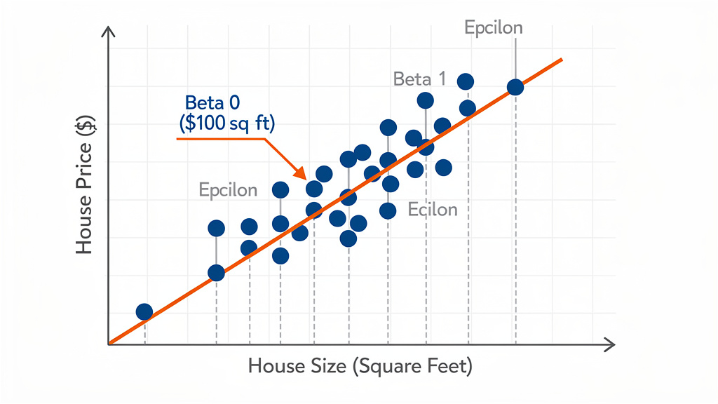
To ground these abstract statistical concepts, consider a concrete real-world scenario: predicting the selling price of residential properties based on their measured living area. When historical transaction data is plotted on a two-dimensional graph—with house size on the horizontal x-axis and sale price on the vertical y-axis—each historical sale appears as an individual point. A visual inspection often reveals an upward trend where larger houses generally command higher prices. While individual properties vary around this trend line, the overall relationship aligns along a linear path.
Mathematically, this relationship is expressed through the simple linear regression formula:
y=β0+β1x+ϵ
Each term in this equation carries a distinct statistical and physical interpretation:
The term y represents the target or dependent variable, which is the numerical value the model seeks to predict (e.g., the final house price in dollars).
The term x represents the input feature or independent variable, which serves as the predictor (e.g., house size in square feet).
The coefficient β0 represents the y-intercept of the regression line. Geometrically, this is the point where the fitted line crosses the vertical axis when x equals zero. In the housing example, β0 represents the theoretical baseline price of a house with zero square feet. Although a zero-square-foot house is physically impossible, the intercept remains mathematically necessary to anchor the regression line in space.
The coefficient β1 represents the slope of the regression line. It quantifies the expected change in the target variable y for every one-unit increase in the predictor variable x. The magnitude and sign of β1 indicate both the strength and the direction of the relationship.
The term ϵ represents the error term or residual. In real-world data, data points rarely fall perfectly along a single straight line. The error term accounts for the vertical difference between an actual observed data point and the value predicted by the regression line. It captures random noise, unmeasured variables, and unpredictable market fluctuations that fall outside the model’s scope.
Interpreting Coefficients with a Practical Example
To make these mathematical symbols concrete, imagine a housing dataset where fitting a linear regression model yields a y-intercept β0 equal to $100,000 and a slope coefficient β1 equal to $110 per square foot.
In this scenario, the intercept indicates a baseline valuation of $100,000. The slope indicates that each additional square foot of living space adds an estimated $110 to the house price. For instance, if a house size increases from 1,000 square feet to 1,100 square feet—a difference of 100 square feet—the model predicts a price increase of 100 times $110, which equals $11,000.
Evaluating the slope coefficient provides valuable domain insights into market dynamics. A steeper slope, such as β1 equal to $300 per square foot, would indicate that living space is highly prized, a condition typical of expensive dense urban environments. Conversely, a shallower slope reflects a market where square footage plays a less dramatic role in driving price.
The error term ϵ represents real-world deviations from these average predictions. For example, if the model predicts a price of $210,000 for an 800-square-foot house, but the actual house sold for $219,000, the residual error is positive $9,000. Conversely, if a home sold for $9,000 less than predicted, the error is negative. These errors stem from factors unmeasured by simple square footage, such as recent renovations, scenic views, or seller urgency.
Dual Objectives: Prediction and Inference
Linear regression serves two major analytical purposes in data science: prediction and statistical inference.
In predictive modeling, the goal is to deploy the trained regression equation to estimate outcomes for new, unseen data inputs. Once the parameters β0 and β1 are established from historical data, predicting the value of a new observation requires simply plugging in the new input value x. For example, if a homeowner wants to estimate the value of a 1,300-square-foot or 1,800-square-foot house, substituting those values into the fitted equation yields an immediate, quantitative price prediction.
In statistical inference, the primary goal is to understand the nature of the relationship between variables. Analysts examine the sign and magnitude of the slope parameter β1 to draw conclusions. A positive slope confirms that increasing the input variable boosts the output variable, whereas a negative slope demonstrates an inverse relationship. Comparing slope magnitudes across different segments or regional markets allows researchers to measure relative feature sensitivity.
Cross-Industry Applications
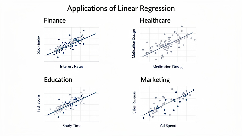
The mathematical framework of linear regression extends far beyond real estate valuation. Virtually any domain where a continuous target variable depends on measurable inputs can leverage regression modeling:
In finance, analysts model stock market indices or asset returns against key economic drivers such as benchmark interest rates or gross domestic product growth metrics.
In healthcare and medicine, clinical researchers study patient recovery outcomes by modeling recovery duration against variables like drug dosage levels or physical therapy hours.
In education, administrators and researchers analyze student academic performance on standardized examinations as a function of dedicated study time or classroom attendance hours.
In marketing, business executives evaluate advertising effectiveness by modeling sales revenue generation against promotional expenditure across various media channels.
Key Limitations and Assumptions
Despite its clarity and widespread applicability, simple linear regression carries fundamental limitations that practitioners must recognize.
First, the model inherently assumes a strict linear relationship between input x and output y. If the true underlying relationship is non-linear—such as an exponential growth curve or an inverted U-shape reflecting diminishing returns—a simple straight line will systematically miscalculate predictions.
Second, relying on a single predictor variable often severely restricts predictive accuracy. Complex real-world outcomes are rarely driven by one factor alone. Omitting important variables leaves a large portion of variance unexplained, resulting in higher residual errors. Furthermore, simple linear regression cannot capture interaction effects where the impact of one variable depends on the state of another.
Finally, standard linear regression assumes homoscedasticity, meaning the variance of the error term ϵ remains constant across all levels of the predictor variable x. In practice, variability often expands as the predictor grows; for instance, price variance among high-end 5,000-square-foot luxury mansions is typically much larger than variance among 800-square-foot starter homes. When these assumptions are violated, transitioning to multiple linear regression or non-linear models becomes necessary.