Multiple Linear Regression: A Comprehensive Guide to Predictive Modeling
Extending simple linear regression into a multidimensional framework for modeling complex real-world phenomena.
In the world of data science and statistical analysis, few techniques are as foundational and widely applicable as multiple linear regression. This powerful method extends the simplicity of basic linear regression into a multidimensional framework, allowing analysts and researchers to model complex real-world phenomena with remarkable accuracy. Whether you are predicting house prices, evaluating patient outcomes, or optimizing marketing strategies, multiple linear regression provides a robust foundation for understanding how multiple factors simultaneously influence a single outcome.
From Simple to Multiple: The Evolution of Linear Regression
Simple linear regression has long been the starting point for anyone learning predictive modeling. In its most basic form, it examines the relationship between a single predictor variable and an outcome variable. For example, you might predict house prices based solely on the size of the house in square footage. The model produces a straight line that best fits the data, minimizing the sum of squared errors between predicted and actual values.
However, the real world rarely operates on single variables. House prices, for instance, are influenced not just by size but by age, location, number of bedrooms, neighborhood quality, and countless other factors. This is where multiple linear regression enters the picture. Instead of relying on one predictor, this technique incorporates several input variables simultaneously to create a more accurate and nuanced model.
The mathematical formulation is elegant in its simplicity. The model takes the form:
y=β0+β1x1+β2x2+β3x3+⋯+βnxn+ϵ
Here, y represents the outcome variable, β0 is the intercept, each βi is the coefficient associated with predictor xi, and ϵ represents the error term. The goal remains the same as in simple linear regression: find the values of the beta coefficients that minimize the sum of squared errors. This is typically solved using linear algebra, and modern software handles these calculations automatically, regardless of how many predictors you include.
Visualizing Multiple Linear Regression
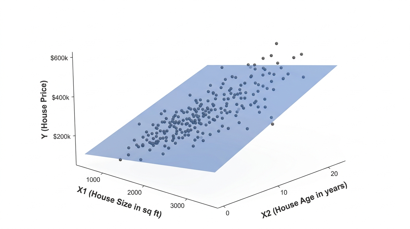
When you move from one predictor to two, the visualization shifts from a two-dimensional line to a three-dimensional plane. With three or more predictors, the model exists in higher-dimensional space as what mathematicians call a hyperplane. While we cannot easily visualize dimensions beyond three, the mathematical principles remain consistent.
The image above illustrates a three-dimensional scatter plot where house price is predicted using both house size and house age. The translucent blue regression plane cuts through the scattered data points, representing the model’s predictions across the range of both input variables. You can observe how the plane slopes upward with increasing house size and downward with increasing house age, capturing the dual influence of these predictors on price.
Interpreting Coefficients: The “Holding Others Fixed” Principle
One of the most important concepts in multiple linear regression is how to interpret the coefficients. Each coefficient represents the estimated change in the outcome variable for a one-unit increase in its corresponding predictor, holding all other variables constant. This principle is often described as “holding others fixed.”
For example, if the coefficient for house size is 150, this means that for every additional square foot, the house price increases by $150, assuming the age of the house and all other variables remain unchanged. Similarly, if the coefficient for house age is -2,000, this indicates that for each additional year of age, the house price decreases by $2,000, holding size and other factors constant.
This isolation of effects is what makes multiple regression so powerful. In the real world, variables are often correlated with each other. Older houses might tend to be smaller, or houses in certain locations might be both larger and newer. A simple regression using only house size would conflate these effects, potentially producing misleading results. Multiple regression controls for these correlations, allowing you to assign the unique influence of each factor to the prediction.
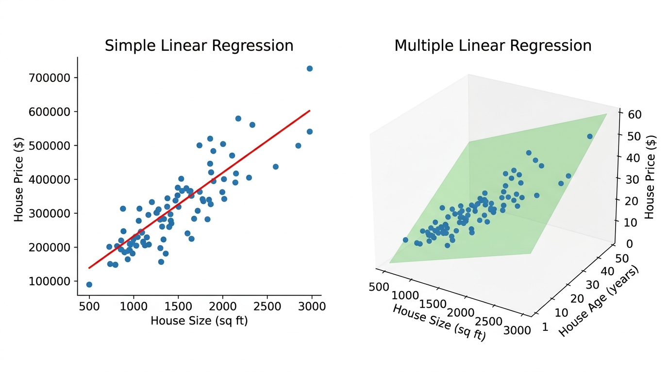
The comparison image above demonstrates this distinction clearly. On the left, a simple linear regression uses only house size to predict price, producing a single line through a two-dimensional scatter plot. On the right, multiple linear regression incorporates both house size and house age, producing a regression plane in three-dimensional space. The multiple regression model captures significantly more of the variation in the data, resulting in tighter predictions and smaller errors.
Why Multiple Predictors Matter
The primary motivation for using multiple predictors is improved prediction accuracy. In a typical example, a simple linear regression using only house size might achieve an R-squared value of around 83 percent. This means the model explains 83 percent of the variation in house prices. While respectable, this leaves 17 percent unexplained. By adding variables such as house age and location, the R-squared value can increase substantially, and the predictions become significantly tighter, with data points clustering more closely around the regression plane.
Beyond accuracy, multiple regression helps address the problem of correlated predictors. When variables are related to each other, simple models can confuse their individual effects. For instance, if older houses tend to be smaller, a model using only size might underestimate the true effect of size on price because it is inadvertently capturing the negative effect of age as well. Multiple regression disentangles these relationships, providing a clearer picture of each variable’s unique contribution.
Evaluating Predictor Importance
When you have multiple predictors, a natural question arises: which ones matter most? Is house size more important than house age? There are several approaches to answering this question.
One common method is to measure the improvement in R-squared when adding each new feature to the model. If adding house age to a model that already includes house size increases R-squared by a significant margin, that suggests age is an important predictor. Another approach is cross-validation, where you systematically add and remove predictors to see how the model’s performance changes on unseen data.
Standardized coefficients also provide insight into relative importance. When all variables are scaled to the same units, the magnitude of each coefficient reflects its relative influence on the outcome. However, this approach should be used cautiously, as it can be sensitive to correlations between predictors.
Real-World Applications
The applications of multiple linear regression extend far beyond real estate. In healthcare, researchers use it to predict patient outcomes based on treatment type, drug dosage, patient age, pre-existing conditions, and lifestyle factors. In marketing, analysts model sales as a function of advertising spend across different channels, seasonality, product pricing, and competitive activity. In transportation, engineers predict fuel efficiency using engine size, vehicle weight, aerodynamic design, and driving conditions.
The key insight is that most outcomes we care about depend on multiple factors. Rarely does a single variable tell the whole story. Multiple linear regression provides a framework for capturing these complex relationships in a way that is both interpretable and actionable.
Guarding Against Overfitting
While adding more predictors generally improves model performance, there is a critical caveat: overfitting. When you include too many variables, especially relative to the amount of data you have, the model can start fitting random noise rather than genuine patterns. This results in a model that performs well on the training data but poorly on new, unseen data.
Cross-validation is one of the most effective tools for guarding against overfitting. By repeatedly training the model on subsets of the data and testing it on held-out portions, you can assess whether adding more predictors genuinely improves generalization or merely memorizes the training set. Other techniques include regularization methods like ridge regression and lasso, which penalize overly complex models, and information criteria like AIC and BIC, which balance model fit against complexity.
Conclusion
Multiple linear regression is a remarkably powerful and versatile tool for understanding complex relationships and making predictions. By extending the simple linear regression framework to accommodate multiple predictors, it allows analysts to model real-world phenomena with greater accuracy and nuance. The principle of “holding others fixed” provides clear, interpretable insights into the unique contribution of each variable, while techniques like cross-validation ensure that models generalize well to new data.
For anyone beginning their journey into predictive modeling, multiple linear regression is an excellent starting point. It is intuitive, computationally efficient, and provides a solid foundation for understanding more advanced techniques. As the transcript emphasizes, most outcomes depend on multiple factors, and multiple regression offers a principled way to capture those relationships. Whether you are analyzing housing markets, optimizing business strategies, or advancing scientific research, multiple linear regression remains an indispensable tool in the data scientist’s toolkit.